CNN과 날씨 이미지를 사용하여 다중 분류를 했다.
결과적으로 5개 종류의 날씨 이미지 30장 중 21장을 정확히 예측했다.
이미지 미리 보기

cloudy, foggy, rainy, shine, sunrise 총 5개 종류의 날씨 이미지가 있으며 alien_test는 예측할 이미지다.
각 날씨의 이름으로 된 폴더에 저장되어 있는 이미지를 하나씩 가져와서 확인해 봤다.
이미지 데이터셋 만들기
이미지를 array 형태로 만드는 것은 복잡하다.
def img_read_resize(img_path): "이미지 읽기, 채널 변경, resize" img = cv2.imread(img_path) img = cv2.cvtColor(img, cv2.COLOR_BGR2RGB) img = cv2.resize(img, (120, 120)) return img
먼저 이미지를 읽어 RGB 채널로 변경하고 120x120 사이즈로 변경하여 반환하는 함수를 만든다.
각각의 이미지마다 크기가 달라 크기를 균일화시키는 것이다.
def img_folder_read(img_label): "특정 날씨 폴더의 전체 이미지 파일을 읽어서 list 에 담아주는 함수" img_files = [] labels = [] img_path = sorted(glob.glob(f"{root_dir}/{img_label}/*")) for ipath in img_path: try: img = img_read_resize(ipath) # 배열 형태로 변경된 이미지 img_files.append(img) labels.append(img_label) except: continue return img_files, labels
특정 날씨 이름을 인자로 주면 해당 날씨 폴더의 전체 이미지를 읽어 img_files 리스트에 담고, 날씨 이름은 labels 리스트에 담아 반환하는 함수이다.
glob에 활용하는 경로는 이미지셋을 저장한 경로에 맞게 지정한다.
img_files, labels = img_folder_read('alien_test') len(img_files), len(labels), labels[0] # 실행 결과 (30, 30, 'alien_test')
함수 테스트 결과 alient_test 폴더의 이미지 30개가 잘 저장된 것을 확인했다.
# 전체 이미지 파일 불러오기 x_train_img = [] x_test_img = [] y_train_img = [] y_test_img = [] # tqdm 을 통해 이미지를 읽어오는 상태를 표시 for img_label in tqdm.tqdm(image_label): img_files, labels = img_folder_read(img_label) if img_label != 'alien_test': x_train_img.extend(img_files) y_train_img.extend(labels) else: x_test_img.extend(img_files) y_test_img.extend(labels) # 실행 결과 100% 6/6 [00:24<00:00, 4.06s/it]
날씨가 담긴 리스트 lmg_label을 순회하며 전체 이미지 파일을 불러온다. for loop의 진행 상황을 확인하기 위해 tqdm을 사용했다.
len(x_train_img), len(x_test_img), len(y_train_img), len(y_test_img) # 실행 결과 (1498, 30, 1498, 30)
전체 train 데이터 1498개 이미지, test 데이터 30개 이미지와 그 레이블을 잘 저장했다.
x_train_img[0].shape # 실행 결과 (120, 120, 3)
리스트에 저장된 이미지는 120x120, 3채널이다.
x, y값을 np.array 형식으로 변환
x_train_array = np.array(x_train_img) y_train_array = np.array(y_train_img) x_test_array = np.array(x_test_img) y_test_array = np.array(y_test_img)
모두 처리를 위해 np.array 형식으로 변환한다.
x_train_array.shape, x_test_array.shape # 실행 결과 ((1498, 120, 120, 3), (30, 120, 120, 3))
x가 잘 변환되었고
y_train_array.shape, y_test_array.shape # 실행 결과 ((1498,), (30,))
x의 레이블인 y도 잘 변환되었다.
random_number = np.random.choice(range(1, 1498), 10) fig, ax = plt.subplots(2, 5) for i, number in enumerate(random_number): ax[i//5][i%5].imshow(x_train_array[number]) ax[i//5][i%5].set_title(y_train_array[number]) ax[i//5][i%5].axis('off')
랜덤으로 10장을 선택하여 imshow로 이미지를 확인해 본다.
자연이 느껴지는 이미지들과 그 레이블을 확인할 수 있다.
train set, valid set 생성
x_train_raw, x_valid_raw, y_train_raw, y_valid_raw = train_test_split( x_train_array, y_train_array, stratify=y_train_array, test_size=0.33, random_state=42)
train : valid = 2 : 1로 분할하며 클래스 비율은 유지한다.
x_train = x_train_raw / 255 x_valid = x_valid_raw / 255 x_test = x_test_array / 255
값을 255로 나누어 0~1의 값으로 정규화한다.
x_train[0] # 실행 결과 array([[[0.03529412, 0.12941176, 0.30196078], [0.03921569, 0.13333333, 0.30588235], [0.03921569, 0.13333333, 0.30588235], ..., [0.08627451, 0.19215686, 0.36862745], [0.08235294, 0.18823529, 0.36470588], [0.08627451, 0.18039216, 0.36078431]], [[0.03529412, 0.12941176, 0.30196078], [0.03921569, 0.13333333, 0.30588235], [0.03921569, 0.13333333, 0.30588235], ..., [0.08627451, 0.19215686, 0.36862745], [0.08235294, 0.18823529, 0.36470588], [0.08627451, 0.18039216, 0.36078431]], [[0.03921569, 0.12941176, 0.30196078], [0.04705882, 0.1372549 , 0.30980392], [0.04705882, 0.14117647, 0.32156863], ..., [0.09019608, 0.19607843, 0.38039216], [0.09019608, 0.19607843, 0.38039216], [0.08235294, 0.18823529, 0.36470588]], ..., [[0.22745098, 0.28627451, 0.33333333], [0.18823529, 0.21176471, 0.30588235], [0.38039216, 0.38431373, 0.47058824], ..., [0.29803922, 0.30588235, 0.35686275], [0.53333333, 0.54117647, 0.59215686], [0.47843137, 0.48627451, 0.53333333]], [[0.18431373, 0.21960784, 0.30196078], [0.37647059, 0.40392157, 0.47843137], [0.15294118, 0.18823529, 0.25490196], ..., [0.46666667, 0.47843137, 0.52156863], [0.43137255, 0.43529412, 0.51764706], [0.34117647, 0.35294118, 0.42745098]], [[0.30980392, 0.34509804, 0.42745098], [0.41960784, 0.44313725, 0.51764706], [0.25098039, 0.2627451 , 0.36470588], ..., [0.55686275, 0.56862745, 0.61568627], [0.51764706, 0.5254902 , 0.57647059], [0.53333333, 0.54901961, 0.60784314]]])
정규화가 잘 적용되었다.
One Hot Encoding
from sklearn.preprocessing import LabelBinarizer lb = LabelBinarizer() lb.fit(y_train_raw) y_train = lb.transform(y_train_raw) y_valid = lb.transform(y_valid_raw) y_train.shape, y_valid.shape, lb.classes_ # 실행 결과 ((1003, 5), (495, 5), array(['cloudy', 'foggy', 'rainy', 'shine', 'sunrise'], dtype='<U7'))
scikit-learn의 LabelBinarizer를 사용하여 클래스 개수 5개에 따라 원핫인코딩 된 결과를 확인할 수 있다.
y_train_raw[:5], y_train[:5] # 실행 결과 (array(['shine', 'shine', 'cloudy', 'shine', 'sunrise'], dtype='<U7'), array([[0, 0, 0, 1, 0], [0, 0, 0, 1, 0], [1, 0, 0, 0, 0], [0, 0, 0, 1, 0], [0, 0, 0, 0, 1]]))
예시로 5개만 출력한 결과
CNN 모델 구성
from tensorflow.keras.models import Sequential from tensorflow.keras.layers import Conv2D, MaxPooling2D, Dense, Flatten, Dropout
모델 구성에 필요한 함수들을 먼저 로드한다.
num_classes = y_train.shape[1] # 5 model = Sequential() # 입력층 model.add(Conv2D(filters=16, kernel_size=(3,3), activation='relu', input_shape=x_train[0].shape)) model.add(Conv2D(filters=16, kernel_size=(3,3), activation='relu')) model.add(MaxPooling2D(2,2)) model.add(Conv2D(filters=16, kernel_size=(3,3), activation='relu')) model.add(Conv2D(filters=16, kernel_size=(3,3), activation='relu')) model.add(MaxPooling2D(2,2)) model.add(Dropout(0.2)) # Fully-connected layer model.add(Flatten()) model.add(Dense(units=128, activation='relu')) # 출력층 model.add(Dense(num_classes, activation='softmax'))
필터 크기가 3x3인 convolution을 2회 한 효과는 5x5인 convolution 1회와 작용이 같다.
그러나 활성화함수 relu를 두 번 사용하여 비선형성이 더 추가될 수 있어서 이 방법이 선호된다.
출력층의 활성화함수는 다중 분류이므로 softmax를 지정했다.
모델 컴파일
model.compile(optimizer="adam", loss="categorical_crossentropy", metrics=["accuracy"] )
모델 fit 하기 전에 옵티마이저(Optimizer), 손실 함수(Loss function), 평가 지표(Metrics) 설정이 컴파일 단계에서 추가된다.
one-hot 형태의 클래스를 예측해야 하므로 손실 함수에 categorical_crossentropy를 지정한 특징이 있다.
모델 fit
from tensorflow.keras.callbacks import EarlyStopping earlystop = EarlyStopping(monitor="val_accuracy", patience=5, verbose=1) history = model.fit(x_train, y_train, validation_data=(x_valid, y_valid), epochs=100, callbacks=earlystop)
epoch는 100이지만 5회 이상 val_accuracy가 개선되지 않으면 학습을 조기 종료하도록 earlystop을 지정했다.
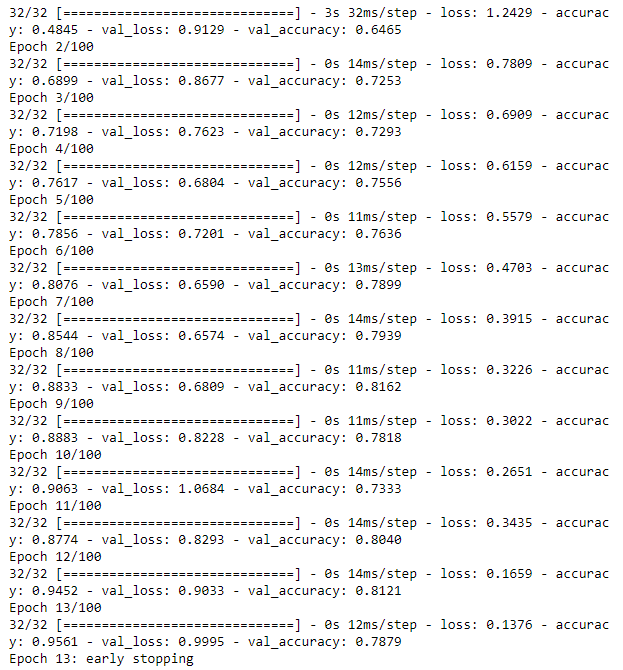
epoch 100에 도달하지 못하고 13에서 early stop 되었다.
history를 데이터프레임으로 만들어 확인하면 아래와 같다.
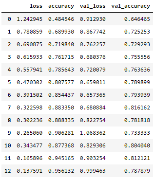
뒤로 갈수록 약간 과적합되는 경향이 보인다.
예측, 실제값과 비교
y_pred = model.predict(x_test) y_predict = np.argmax(y_pred, axis=1) y_predict # 실행 결과 array([1, 2, 0, 0, 1, 0, 0, 4, 0, 0, 1, 4, 1, 2, 2, 2, 2, 2, 2, 2, 3, 3, 3, 4, 4, 4, 4, 4, 4, 4])
예측해야 하는 30개의 이미지에 대한 예측값이다.
30개 이미지와 정답 여부를 출력해 보면
fig, axes = plt.subplots(6, 5, figsize=(20, 20)) for i, xt in enumerate(x_test): row = i // 5 col = i % 5 color = "b" if y_test[i] != y_predict[i]: color = "r" axes[row][col].imshow(xt) axes[row][col].set_title(f"{test.loc[i, 'Image_id']}, {lb.classes_[y_predict[i]]}", c=color) axes[row][col].axis('off')
정답일 경우 타이틀이 파란색, 오답일 경우 타이틀이 빨간색으로 출력되도록 했다.
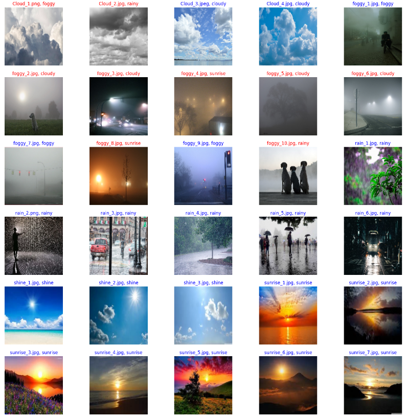
CNN을 이용한 날씨 이미지 다중 분류 결과 30개 중 21개 정답, 9개 오답이 나왔다.
사람이 눈으로 보기에도 틀릴 만한 것들에서 오답이 나온 것 같다.
'AI SCHOOL > TIL' 카테고리의 다른 글
| [DAY 81] Week 18 Last Insight Day 미드프로젝트2 리뷰 리포트 (0) | 2023.04.20 |
|---|---|
| [DAY 80] Bidirectional RNN을 통해 삼성전자 주가 예측하기 (0) | 2023.04.19 |
| [DAY 78] CNN과 이미지 데이터를 활용한 말라리아 감염 여부 이진 분류 예측 (0) | 2023.04.17 |
| [DAY 77] 코딩테스트 연습 - 정규표현식, 페이지 교체 알고리즘, 카카오 문제 (0) | 2023.04.14 |
| [DAY 76] Week 17 Insight Day 미니프로젝트5 시작, Resume & Portfolio 특강 (0) | 2023.04.13 |


댓글